The presentation of data is considered to be just as important as the data analysis itself. In this blogpost we will look at 5 examples from Ron Cody’s “Learning SAS by Example: A Programmer’s Guide” which will help us summarize data and create meaningful reports out of it. The main topics we will cover are as follows –

1. Summarizing Data
2. Counting the Frequencies
3. Creating Tabular Reports

The format we will follow for each problem is quite similar to my previous blogpost and it is as follows -

1. Problem
2. Code
3. Result
4. Learning

Summarizing the data

In this section we will try to understand how Proc Means can be used to summarize data using various commands

1) Using the SAS data set College (available in the link at the bottom), we will report the mean GPA for the following categories of ClassRank: 0–50 = bottom half, 51–74 = 3rd quartile, and 75 to 100 = top quarter. This is done by creating an appropriate format. We will not use a DATA step.

Code

In the first proc step, we are creating the 3 constrains and naming them accordingly which will serve as the 3 row names in the result. In the second proc step we first declare what descriptive analysis we need to do, in this case n and mean. Later we are specifying how they will be categorized by using CLASS function instead of a BY function. var stands for variable. It tells SAS which variable to be taken for analysis.

Result

Learning

In this exercise we have learnt how to use descriptive statistics related to Proc Means and classify that data based on the desired variables. 

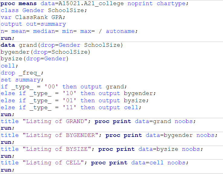
2) Using the SAS data set College we will create four summary data sets containing the number of non-missing and missing values and the mean, minimum, and maximum for ClassRank and GPA, broken down by Gender and SchoolSize. The first data set (Grand) will contain the statistics for all subjects, the second data set (ByGender) will contain the statistics broken down by Gender, the third data set (BySize) will contain the statistics broken down by SchoolSize, and the fourth data set (Cell) will contain the statistics broken down by Gender and SchoolSize. We will do this by using PROC MEANS (with a CLASS statement) and one DATA step. 

Code

 In the first proc step we are, like in the previous example, using proc means and categorizing it with CLASS function. Then var is used to select variables. the functions within means are in the 5th line. In the Data step, drop is used to remove the two variables Gender and SchoolSize. We are actually doing a triple activity in a single data step(as shown in chapter 8) In the end we are using an IF - ELSE statement to get the desired output.   

Result

Learning

In this exercise, we have learnt firstly how to create multiple tables in a single data step. Secondly, how to effectively use  If - Else statements to fill in every table by the requirement 

Counting the Frequencies

In this topic we will try to understand how Proc Freq can be used for the purpose of creating meaningful tables to summarize the data.

3) Using the data set Blood, we will produce frequencies for the variable Chol (cholesterol) using a format to group the frequencies into three groups: low to 200 (normal), 201 and higher (high), and missing. We will run PROC FREQ twice, once using the MISSING option, and once without to compare the percentages in both listings.

Code

 In the first step, proc format, we use value function to categorize chol into 3 segments i.e Normal, High, and Missing(for missing values). In the second step, proc freq we find the frequencies taking into consideration the missing values. In the third step, we find the frequencies without considering the missing values. 

Result

Learning

In this exercise we learn how to get rid of the missing values with ease using different types of formatting techniques.

Creating Tabular Reports

In this section we will learn how to create tables having multiple variables in both columns and rows. This is largely used to create descriptive statistics for final reports

   

4) We will produce the following table.

Result

 Code

In the first step, we format the variables into 2 sections by Gender. Next we use proc tabulate create a table using Class function and 3 variables. Next we use tables function to multiply Gender and Scholarship to get the desired result.

Learning

We have learnt here how to create tabular reports using proc tabulate. This has helped us summarize the data in one single table instead of multiple tables.

5) We are trying to produce the following table. 

Result

Code 

Learning

We have learnt how to use descriptive statistics in the tabular format. This is used for reporting research studies.

The following is the link to access the data sets and the code used to create this blogpost - https://drive.google.com/file/d/0B2sVurZ_f97PSWwyQW9aZEFhdk0/view?usp=sharing 

SAS Overview

                         SAS at the first glance may seem like an alien language, especially for someone with a non coding background (like me), but sooner than later you will start to realize that it is quite close to 'English' and suprisingly enough fun to learn, taking into consideration its user - friendly interface and English like syntax. Today I would like to use this opportunity to take you through 10 different problems in SAS from the book "Learning SAS by Example: A Programmers Guide" by Ron Cody using 'SAS University Edition'. The topics we will be covering are as follows-

1) Conditional Processing
2) Iterative Processing : Looping
3) Working with Dates
4) Subsetting and Combining 
5) Working with Numeric Functions


The format I will be following here is as follows -
1) The problem statement
2) Then, the code that I have used in SAS Studio
3) The output displayed
4) Finally, what have we got to learn from it.

Conditional Processing

Question 1 (Chapter 7 Prob 1)

Using IF and ELSE IF statements, we will compute two new variables as follows:
Grade (numeric), with a value of 6 if Age is 12 and a value of 8 if Age is 13. The quiz grades have numerical equivalents as follows: A = 95, B = 85, C = 75,  D = 70, and F = 65. Using this information, we compute a course grade (Course) as a weighted average of the Quiz (20%), Midterm (30%) and Final (50%). 

Code -

Result -

Learning - We have learnt here to use If Else function along with the method to find Weighted Average.

Question 2 (Chapter 7 Prob 7)

We are provided with a data set by the name 'Bicycles'. The variables of the data set are as follows-
Country
Model
Manufacturer
Units
Unit Cost
Total Sales

Using the Bicycles data set, we will list all the observations for Road Bikes that cost more than $2,500 or Hybrids that cost more than $660. The variable Model contains the type of bike and UnitCost contains the cost.

Code -

Result -

Learning - In this program we have learnt how to use where and or function in the proc print data step to filter out data.

Iterative Processing : Looping

Question 3 (Chapter 8 Prob 3)

Let us modify the program here so that each observation contains a subject number (Subj), starting with 1: 


Code -

Result -

Learning - We have learned to add a new Column into the output without using datalines or DO loop.



Question 4 (Chapter 8 Prob 5)

We will now create and print a data set with variables N and LogN, where LogN is the natural log of N (the function is LOG). Then, we will use a DO loop to create a table showing values of N and LogN for values of N going from 1 to 20. 

Code -












Result -


























Learning - We have learnt here how to use DO loop with reference to Logarithm function.

Working with Dates

Question 5 (Chapter 9 Prob 1)

We have several lines of data, consisting of a subject number and two dates (date of       birth and visit date). 
The subject starts in column 1 (and is 3 bytes long), 
The date of birth starts in column 4 and is in the form mm/dd/yyyy, 
The visit date starts in column 14 and is in the form nnmmmyyyy
The lines of data to create a temporary SAS data set called Dates.Let us format both dates using the DATE9. format and include the subject’s age at the time of the visit in this data set. 
0011021195011Nov2006    
0020102195525May2005    
0031225200525Dec2006 

Code -

Result -

Learning - Here we have learned to play around with dates. Firstly, we learned to format dates into 2 different formats. Second, we have learned to find the difference between two dates and consequently compute the Age. 



Question 6 (Chapter 9 Prob 4)

We are given a dataset named Hosp. Using the Hosp data set, we will compute the subject’s ages two ways: 
As of January 1, 2006 (AgeJan1)
As of today’s date (AgeToday) 
The variable DOB represents the date of birth. We will take the integer portion of both ages and list the first 10 observations.

Code - 












Result -




























Learning - Similar to the previous question, we have used yrdif function, the difference is that this time we have used it twice. Once with today() function to find the age as of today and once age as of 1st Jan 2006 

Sub-setting and Combining

Question 7 (Chapter 10 Prob 1)

We are given a dataset 'Blood'. Using the Blood dataset,we will create two temporary SAS data sets called Subset_A and Subset_B. In both of these data sets we will include a variable called Combined equal to .001 times WBC plus RBC. Subset_A will consist of observations from Blood where Gender is equal to Female and BloodType is equal to AB. Subset_B will consist of all observations from Blood where Gender is equal to Female, BloodType is equal to AB, and Combined is greater than or equal to 14.

Code -



Result - 

Learning - In this program, we have learned how to use subsetting to split a data set into 2 or more sets using a single datastep and at the same time keep the subsetting conditional. 



Question 8 (Chapter 10 Prob 7)

We are given a dataset Using the Gym data set, we create a new, temporary SAS data set (Percent) that contains all the variables found in Gym plus a new variable (CostPercent) that represents the Cost as a percentage of the average cost for all subjects. Using PROC MEANS to create a SAS data set containing the mean cost, we will round this value to the nearest percent.

Code -

Result - 

Learning - We have now learnt how to first calculate average, then using that find the percentage of the observation based on the average.

Working with Numeric Functions

Question 9 (Chapter 11 Prob 1)

We are given a dataset by the name of 'Health'. Using this data set Health, we will compute the body mass index (BMI) defined as the weight in kilograms divided by the height (in meters) squared. We then create four other variables based on BMI: 
1) BMIRound is the BMI rounded to the nearest integer 
2) BMITenth is the BMI rounded to the nearest tenth 
3) BMIGroup is the BMI rounded to the nearest 5 
4) BMITrunc is the BMI with a fractional amount truncated. 
Conversion factors that we are using are: 1 Kg equals 2.2 Lbs and 1 inch = .0254 meters. 

Code -

Result -

Learning - In this program, we have learnt how to round off observations as well as truncate the observations.



Question 10 (Chapter 11 Prob 3)

We again use the Blood dataset to create a new, temporary SAS data set (Miss_Blood). We will set Gender, RBC, and Chol to a missing value if WBC is missing.

Code-

Results -

Learning - In this program we learn how to deal with missing values using 'missing' function as well 'call missing function.

In conclusion, we have learnt a few basic SAS concepts. I hope I have contributed towards some value addition. Thank you for your patience. 

This is the link to the Datasets and SAS codes used in the blogpost -
https://drive.google.com/file/d/0B2sVurZ_f97PTmRPdGN4eU55S3M/view